Real estate mapping
This project uses scraped data to find out tax information on real estate in Mecklenburg County, NC. We can use this data to predict home prices based on historic trends as well as information about the house itself and the surrounding neighborhoods. First we import the data and do some cleaning.
In [1]:
import pandas as pd
import numpy as np
import random as rd
import mpl_toolkits.basemap as bmap
import matplotlib.pyplot as plt
%matplotlib inline
from sklearn.grid_search import GridSearchCV
from sklearn.ensemble import GradientBoostingRegressor
from sklearn.pipeline import Pipeline
from sklearn.preprocessing import Imputer
from sklearn.metrics import mean_squared_error
rd.seed(123)
ch_data = pd.read_csv("/Users/travisbyrum/charlotte_re/new_final_01.csv", dtype={'parcel_id': str})
ch_data.columns
df = ch_data.drop(['land_use', 'land_use', 'neighborhood_code', 'neighborhood', 'land_unit_type', 'property_use_description',
	'foundation_description', 'exterior_wall_description', 'heat_type', 'ac_type', 'three_quarter_baths', 'half_baths',
	'building_type', 'pid_char','deed_book', 'legal_reference'], axis=1)
df['stories'] = df['stories'].str[0].convert_objects(convert_numeric=True)
df['sale_date'] = df['sale_date'].str[6:10].convert_objects(convert_numeric=True)
df = df[df['sale_date'] >= 2000]
df = df[df['sale_price'].notnull()]
df['pct_ch'] = df.groupby(['parcel_id'])['sale_price'].pct_change()
df['pct_ch'].fillna(0, inplace=True)

# Take the log transformation of the price
df['pricelog'] = np.log(df['sale_price'])
with pd.option_context('mode.use_inf_as_null', True):
    df = df.dropna()
After importing the necessary packages, we do some cleaning and transformations to get the data in a workable form.
In [2]:
response = df['pricelog']
df_x = df[df.columns.difference(['parcel_id', 'sale_price','pricelog','pc_ch'])]
train_rows = rd.sample(df.index, int(len(df)*.70))
df_train = df_x.ix[train_rows]
response_train = response.ix[train_rows]
df_test = df_x.drop(train_rows)
response_test = response.drop(train_rows)
Here we set up the training and testing data sets. Currently I am using a 70-30 split between testing and training.
In [3]:
params = {'n_estimators': [100, 300, 500], 'max_depth': [3,5], 'subsample': [1, 0.8],
        'learning_rate': [0.1, 0.05, 0.01], 'loss': ['ls','huber'],'alpha':[0.95]}

model = GradientBoostingRegressor(**params)
gs_cv = GridSearchCV(model, params).fit(df_train, response_train)
After using a grid search for the best parameters values we fit a GBM model to model housing prices.
In [4]:
params = gs_cv.best_params_
model = GradientBoostingRegressor(**params).fit(df_train, response_train)
This fits a model with the best parameters as found through the grid search optimization.
In [5]:
test_score = np.zeros((params['n_estimators'],), dtype=np.float64)
for i, y_pred in enumerate(model.staged_decision_function(df_test)):
    test_score[i] = model.loss_(response_test, y_pred)

plt.figure(figsize=(12, 6))
plt.subplot(1, 2, 1)
plt.title('Deviance')
plt.plot(np.arange(params['n_estimators']) + 1, model.train_score_, 'b-', label='Training Set Deviance')
plt.plot(np.arange(params['n_estimators']) + 1, test_score, 'r-', label='Test Set Deviance')
plt.legend(loc='upper right')
plt.xlabel('Boosting Iterations')
plt.ylabel('Deviance')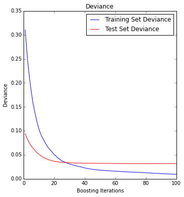
From the deviance plot we see that our test error becomes rather flat with increased boosting iterations.
In [6]:
feature_importance = model.feature_importances_
feature_importance = 100.0 * (feature_importance / feature_importance.max())
sorted_idx = np.argsort(feature_importance)
pos = np.arange(sorted_idx.shape[0]) + .5
plt.figure(figsize=(12, 6))
plt.subplot(1, 1, 1)
plt.barh(pos, feature_importance[sorted_idx], align='center')
plt.yticks(pos, df_train.columns[sorted_idx])
plt.xlabel('Relative Importance')
plt.title('Variable Importance')
plt.show()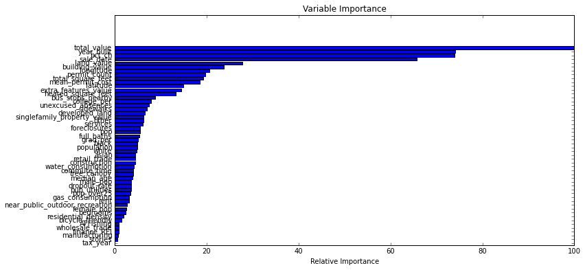
In [7]:
#Grouping houses by their latest sale date
id_pred = df.groupby(['parcel_id'])['sale_date'].transform(max) == df['sale_date']
df_pred = df[id_pred]
df_pred.loc[df_pred.sale_date != 2015, 'sale_date'] = 2015
df_pred = df_pred[df_pred.columns.difference(['parcel_id', 'sale_price', 'pricelog', 'pc_ch'])]
df_pred['predicted_values'] = model.predict(df_pred)
df_pred = df_pred.sort('predicted_values')
In [8]:
def northcarolina_map(ax=None, lat_lleft=34.98,lat_ur=35.55,lon_lleft=-81.15,lon_ur=-80.52):
    new_map = bmap.Basemap(ax=ax, projection='stere',
    lon_0=(lon_ur + lon_lleft) / 2,
    lat_0=(lat_ur + lat_lleft) / 2,
    llcrnrlat=lat_lleft, urcrnrlat=lat_ur,
    llcrnrlon=lon_lleft, urcrnrlon=lon_ur,
    resolution='l')
    new_map.drawstates()
    new_map.drawcounties()
    return new_map
After creating the map for Mecklenburg county we can plot the predicted sale prices geographically according to their latitude and longitude.
In [8]:
plt.figure(figsize=(12, 6))
m = northcarolina_map()
x,y = m(df_pred['longitude'].tolist(),df_pred['latitude'].tolist())
#m.scatter(x,y,c=np.array(df_pred['predicted_values'])/1000,s=60,alpha=0.5,edgecolors='none')
m.scatter(x,y,c=np.array(np.exp(df_pred['predicted_values']))/1000,s=60,alpha=0.5,edgecolors='none')
c = m.colorbar(location='right')
c.set_label("Predicted Sales Price")
plt.show()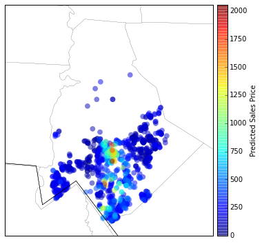
In [9]:
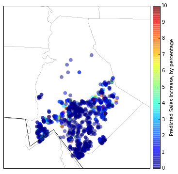
#5 year projection
id_pred = df.groupby(['parcel_id'])['sale_date'].transform(max) == df['sale_date']
year_proj = df[id_pred]
year_proj.loc[year_proj.sale_date != 2015, 'sale_date'] = 2020
year_proj = year_proj[year_proj.columns.difference(['parcel_id', 'sale_price', 'pricelog', 'pc_ch'])]
year_proj['predicted_values'] = model.predict(year_proj)
Here are the sale price projections in five years plotted geographically.
In [10]:
plt.figure(figsize=(12, 6))
m = northcarolina_map()
x,y = m(df_pred['longitude'].tolist(),df_pred['latitude'].tolist())
v = (np.array(np.exp(year_proj['predicted_values']))-np.array(np.exp(df_pred['predicted_values'])))/np.array(np.exp(df_pred['predicted_values']))
m.scatter(x,y,c=v,s=60,alpha=0.5,edgecolors='none', vmin=0, vmax=10)
c = m.colorbar(location='right')
c.set_label("Predicted Sales Increase, by percentage")
plt.show()